OpenStreetMap now provides public access to the access logs of their tile map server from 2014 until today. In this article I will show you how to parse the access logs with Bash and Python and visualize the data with CartoDB.

Prof. Stefan Keller documented the early findings from this analysis on the Geometa Lab Blog.

Many thanks to Matt Amos for making the log files accessible and to @sfkeller and @mrothh for their help.

Total OSM Views

All OSM tile access logs at zoom level 18 aggregated over the period of 2014.

OSM Views over Time

All OSM tile requests per day at zoom level 18 aggregated over the period of 2014 Q1 until 2015 Q1. The CartoDB animation might not work all browsers.

Tile Coordinates

To understand how tiling in OpenStreetMap or Google Maps works you best take look at this visualization from Maptiler and the Google Maps API Docs.

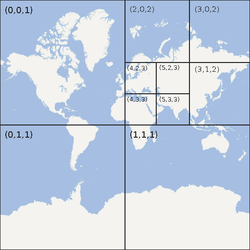
You basically have tiles in the same size (256x256 pixels) and there is one tile at the top (zoom level 0). This tile is divided into 4 other tiles (zoom level 1), then 16 (zoom level 2) and so on. This partitioning strategy is called QuadTiles.

The coordinates in the example below use (x,y,zoom) as format. The index always starts at 0 on the upper left corner.

Download and extract the Tiles

Download all the access logs from the OSM server.

wget -nH -A xz -m http://planet.openstreetmap.org/tile_logs

Now extract the logs (you need to install the XZ Utils first).

unxz *.xz
rm *.xz

Now take a look at one of the log files.

head -n 10 tiles-2015-05-21.txt

The access log has the tile index in the format zoom,x,y in the first column and the number of views for that time period in the second column. Tiles that were not accessed that day or have fewer than 10 views do not appear in the access log file.

0/0/0 588590
1/0/0 139613
1/0/1 116224
1/1/0 135179
1/1/1 114632
2/0/0 138471
2/0/1 181236
2/0/2 109795
2/0/3 68219
2/1/0 182391

We expand tile coordinates into separate columns (from 1/0/0 139613 to 1 0 0 139613).

sed -i 's/\// /g' *.txt

Now that we have valid CSV files we should rename them accordingly (from .txt to .csv).

rename 's/\.txt$/\.csv/' *.txt

You can now import those CSV files into your database. We will continue with plain old Bash and some Python in this article.

Calculate Tile Coordinates

To translate the tiles into actual coordinates we need to convert the tile indizes into coordinates.

The mercantile library allow us to easily calculate the spherical mercator coordinates for tiles.

pip install mercantile

We want to calculate the coordinates for the center of each tile.

def calculate_center(x, y, zoom):
    bounds = mercantile.bounds(x, y, zoom)
    height = bounds.north - bounds.south
    width = bounds.east - bounds.west
    center = (bounds.north + height / 2, bounds.west + width / 2)
    return center

Now we write a stream processing script that reads our prepared CSV from stdin and writes the tiles with the added coordinates to stdout.

cat tiles-2015-05-21.csv | ./calc_coords.py

You can look at the full script here.

Visualize Tile Access over Time

Prepare

Because we have too much data to display it all at once, we will only look at tiles with the zoom level 18 (which means people have zoomed in with a particular interest for that area).

cat tiles-2015-05-21.csv | awk '$1 == "18"'

To cut down the dataset even more we are only interested in tiles with coordinates that are inside a bounding box around Switzerland.

NORTH = Decimal('47.9922193487799')
WEST = Decimal('5.99235534667969')
EAST = Decimal('11.1243438720703')
SOUTH = Decimal('45.6769214851596')

def in_switzerland(coords):
    lat, lng = coords
    return lat < NORTH and lat > SOUTH and lng > WEST and lng < EAST

You can look at the full script here.

Now we can extract all swiss access logs.

cat tiles-2015-05-21.csv | ./filter_switzerland.py

In order to upload them to CartoDB we also need to add the time dimension as first column.

cat tiles-2015-05-21.csv | sed -e "s/^/2015-05-21 /"

Import in CartoDB

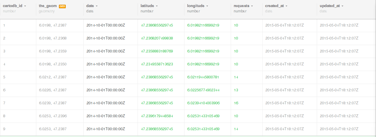
When uploading make sure you have a header row in your CSV. If you call the coordinates latitude and longitude CartoDB will automatically recognize the geometry.

Create Heatmap

Now that the dirty prepartion is over let’s get to the fun part.

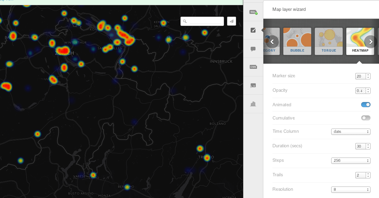
Creating a Heatmap with CartoDB is quite simple. Select the heatmap template and choose the date column as time dimension.

Conclusion

The OSM access logs have alot of interesting datapoints that only wait to be analyzed. The prepartion is dirty work but displaying the data in CartoDB is a breeze. Stay tuned for further analysis.